II: Arrange the Data
In which we rearrange the imported
data so that we can do something useful with it.
6: Expand the Columns
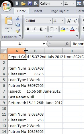
If we double-click on the line between the column headers for columns A
and B, column A will expand to the width of its contents.
We can do the same on the next column too. That way we can see what
we're doing a little better.
7:
Transpose the
First Record
Our data's arranged in useless clumps, and this won't do. We need to
rearrange things if we're going to get anything meaningful out of this
spreadsheet. We can do that by transposing the data so that it reads
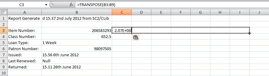
horizontally rather than vertically. Click in cell C3 and type
=TRANSPOSE(B3:B9) followed by Return. Now click on C3 again, and drag the corner
of the box to the right to highlight cells C3 to I3 inclusive.
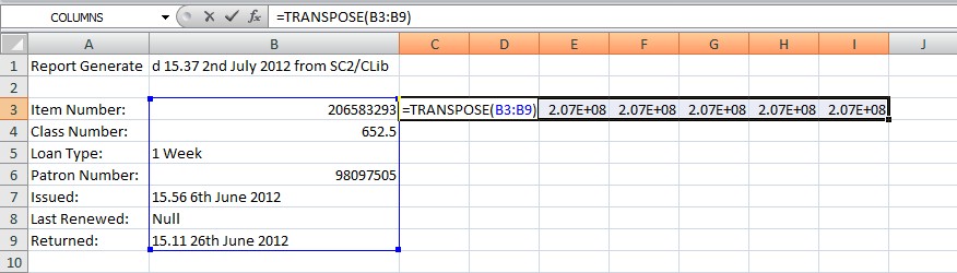
Once we let go we should see content in each of the cells we've just
dragged across. Press the function key F2, and B3:B9 should become
highlighted with a blue border.
Press Ctrl Shift and Return together. Now the contents of C3:I3 should be the same as
the contents of B3:B9.
We have transposed.
8: Expand the
Transposition across All Records
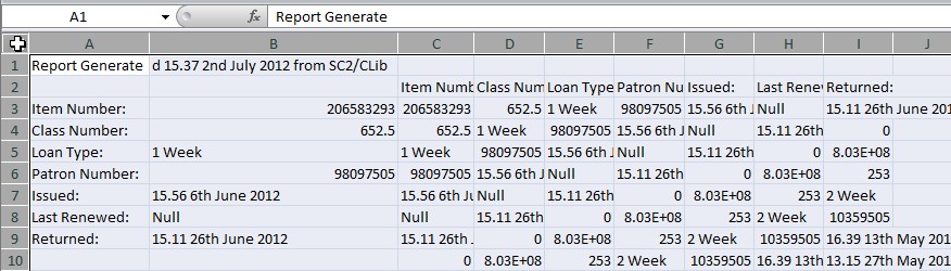
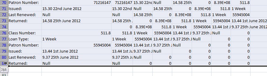
Keeping C3:I3
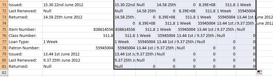
highlighted, drag the bottom right corner of the box down all the way
to the bottom of our data (at row 81) and let go. This will autofill
our transposition all the way down the spreadsheet. Don't worry that it
looks a bit of a mess.
9: Transpose the
Data Labels
Given that we've transposed the data, we should transpose the labels
too. Click on C2 and
repeat what we did at step 7 for the data labels in A3:A9. Don't let any #VALUE! errors put you off as
you do it. If you can't get it to work by doing it yourself, highlight
below for the instructions:
In C2, type =TRANSPOSE(A3:A9).
Click C2 and drag the corner of the box right to highlight cells C2:I2
inclusive. Press F2, then Ctrl Shift and Return together. The labels
should now be transposed.
10:
Repaste the Data
as Values
Now we need to sort out this mess we've created. When we auto-filled
our transposition, we got a lot of useless repetition of data. The only
rows we need are the top rows in each record block: those with the
label Item Number: in
column A. We can safely delete the rest. But we can't delete things
yet, because we have formulae in our transposed cells that are reliant
on some of the stuff we want to get rid of. So let's get rid of that
problem by repasting our data as fixed values. Click in the square to
the left of the header for column A and above the row numbers. This
selects all of our spreadsheet.
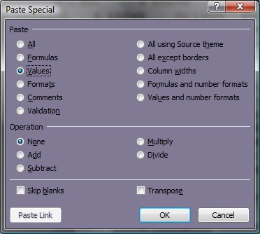
Right click anywhere within the spreadsheet and select "Copy", then right click
again and select "Paste
Special…". We get a dialogue with a whole host of options. We
need to select the radio button for "Values". That done, press "OK".
11: Enable Filters
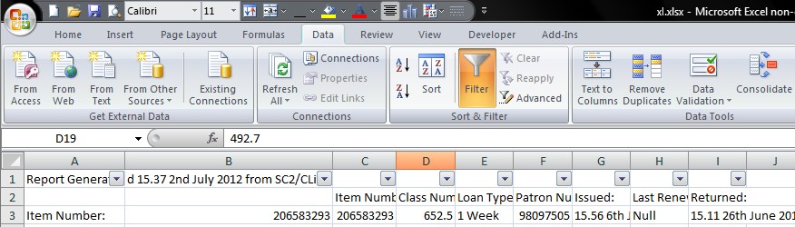
Now we've got rid of any formula reliance we can set about deleting the
data we don't need. With everything in our spreadsheet still selected,
go to the "Data" menu
ribbon and click "Filter"
from the "Sort & Filter"
menu panel. This gives us some little dropdown toggles at the top of
each of our columns.
12: Filter Out a
Record Category
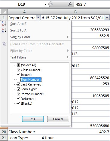
Click the dropdown toggle at the top of column A. This brings up a
dialogue box with a list of data we can filter. Click on the tick next
to "Item Number:" to
unselect it. Everything else in the list should be ticked. Then click
on "OK".
13: Delete Filtered
Data
Our data has now been filtered, and the rows that we want to keep have
been removed from our sight. We don't need the rest of this so we can
delete it: Click on the row number for row 4 and drag down to the end
of our data at row 81.
Right click and select "Delete
Row". Our spreadsheet should now look terrifyingly empty. Go
back to the filter toggle at the top of column A, reselect "Item Number:" and click on "OK". Our beloved data is
back.
14: Move Cells
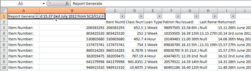
The first two columns are now surplus to requirements. We can start
cleaning that up by moving that pair of cells on the top row. Click A1, hold and drag to B1 and then release to
highlight the two cells. Now click at the middle of the bottom border
of the two cells and drag.
We can drag these cells to anywhere we like, but C14:D14 looks a suitable
enough place. Stick them there.
15: Delete
Unnecessary Columns and Rows
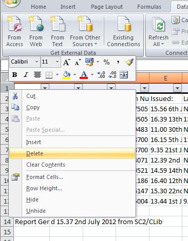
Click on the header for column A and drag right to highlight column B
too. Right click in the selection and click "Delete". Do the same for
row 1.
We should now have Item Number:
in A1.
16: Change the
Column Widths
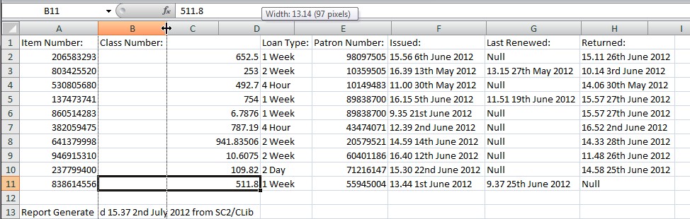
Select everything again with that square to the left of the column A
header, and then double-click on the division between the headers for
column A and column B to neaten things out a bit. The contents of B13 have made our second
column a bit too wide, so click somewhere in the spreadsheet to
unselect everything, then click the border between the headers of
columns B and C and drag left to the colon of Class Number: to make a more
sensible width.
On a normal 1024 resolution display we should now be able to see
everything on the same screen, but it doesn't matter if that's not the
case. It should at least look reasonably sensible at last.
17: Format Leading
Zeroes
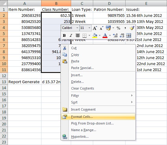
The Dewey references in the "Class Number:" column lack leading
zeroes, and this simply will not do. Select B2:B11, and right click
within the selection. Click on "Format
Cells…".
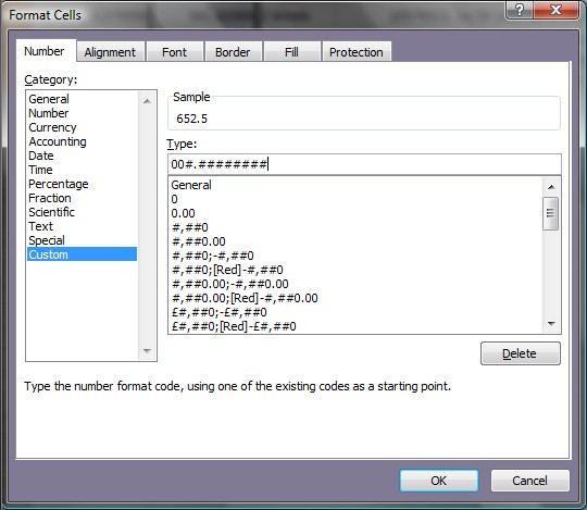
Select "Custom" from
the "Category:" list in
the "Number" tab. In
the text field below where it says
"Type:", delete "General" and write 00#.########
then click "OK".
Our
shelf marks should now look a bit more like they're meant to, and the
hashes there make the formatting good for up to eight decimal places
which is more than we
need right now.