III: Extract the Time
In which we generate an Excel-friendly
Time format from the imported data.
18: Insert Columns
The times and dates within our spreadsheet look very nice, but at
the moment they are just text. We need to persuade Excel to recognize
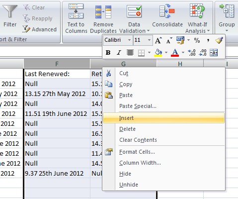
them as dates if we're going to do anything with them. First, highlight
columns F and G, right click in the header and
select "Insert" to give
ourselves two new columns to play with.
19:
Extract a Time
from a Text String using =LEFT
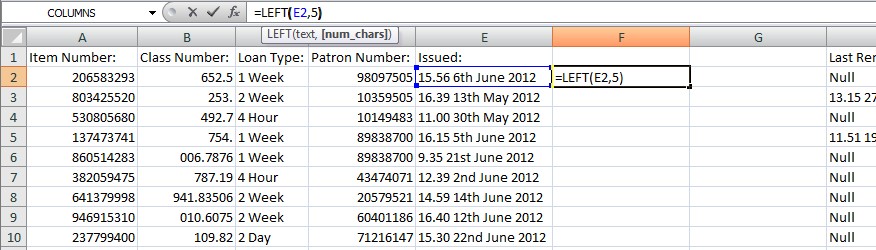
We'll start by extracting the time. Click cell F2 and type
=LEFT(E2,5) . This gives us the
first five characters (from the
left)
within E2.
When we press Return we should get 15.56 displayed in F2.
20: Extract the
Hours of a Time using =QUOTIENT
In G2 type =QUOTIENT(F2,1) ,
then press Return.
This will divide F2 by 1,
and just give
us the bit of the number before the decimal point (i.e. 15).
21: Make Some More
Space
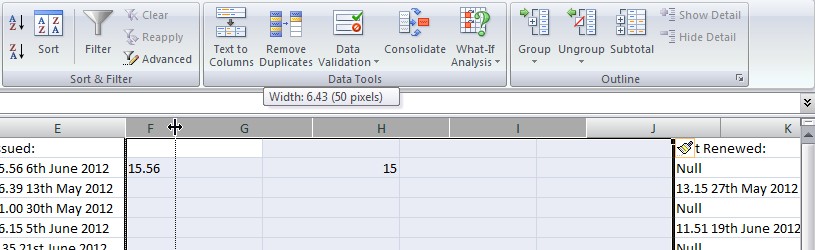
21. Highlight columns H and I, right click and "Insert" another
couple of columns. Highlight F, G, H and I, click between the headers
of F and G and drag to narrow the column widths to something a bit more
friendly. 50 pixels
would be ideal (the width is given in the tooltip).
22: Extract the
Minutes of a Time using =MOD
In H2 type =MOD(F2,1)*100
and press Return.
MOD does the same as QUOTIENT but for
the stuff to the right of the decimal point. Without the multiplication
by 100 it would give us 0.56 here, but instead we should have 56 in this cell.
23: Use the =TIME
function to combine Hours and Minutes
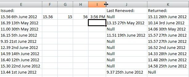
In I2 type =TIME(G2,H2,0)
and press Return.
This will convert the two numbers in G2 and H2 into a
time (with 0
representing the number of seconds). You'll probably have
to expand column I in order to see the result (3:56 PM).
24:
Consolidate the
Formulae into a Single Cell
We can combine all of the above into a
single formula. Click cell F2
again, click in the Formula Bar
at the top, and replace what we wrote
before with:
=TIME(QUOTIENT(LEFT(E2,5),1),MOD(LEFT(E2,5),1)*100,0)
This is simply the formula we wrote in I2, but with the formula we
wrote in G2 in place of
the cell reference for G2
and the formula we wrote in H2
in place of the cell reference for H2.
After pressing Return, double-click on the border between the headers
of
column F and column G to reset the width of F.
25: Delete Redundant
Cell Contents
We can now
delete the contents of G2,
H2 and I2: Click in G2, drag across to I2 and release. Then press the
Delete button to clear the cells.
26:
Extrapolate the
Time Formula for All Records
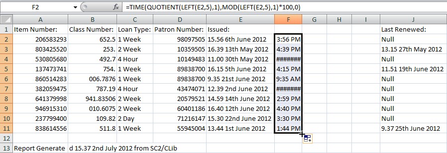
Select cell F2 and drag
the bottom right-hand corner of the cell to
auto-fill F2:F11. We
should now have times for all of our entries, and
they should match the times given in E2.
Adjust the column width again so that all the times display correctly.