IV: Extract the Date
In which we procure an Excel-friendly
date format from the imported data.
27: Extract Text
using =MID
Now let's get the date. Go to G2
and type
=MID(E2,6,LEN(E2)) then press
Return. MID
gives us a section of E2 that (in this case) starts at the sixth
character and goes on for the full length (LEN) of E2. In all cases
except E6, starting at the
seventh character would be preferable (the sixth character is a space
for all entries except E6), but
the ensuing blank space we get at the front will not pose us a problem,
while
mangling the data from E6 definitely would.
28: Remove Ordinals
using =SUBSTITUTE
Excel still won't recognize this as a date because it doesn't like
our use of ordinals. We need to get rid of them.
In H2 type
=SUBSTITUTE(G2,"th","")
and press Return. This will find any "th" in G2 and replace it
with nothing.
But we'll also need to extract "st",
"nd" and "rd", so
let's factor those into our formula too:
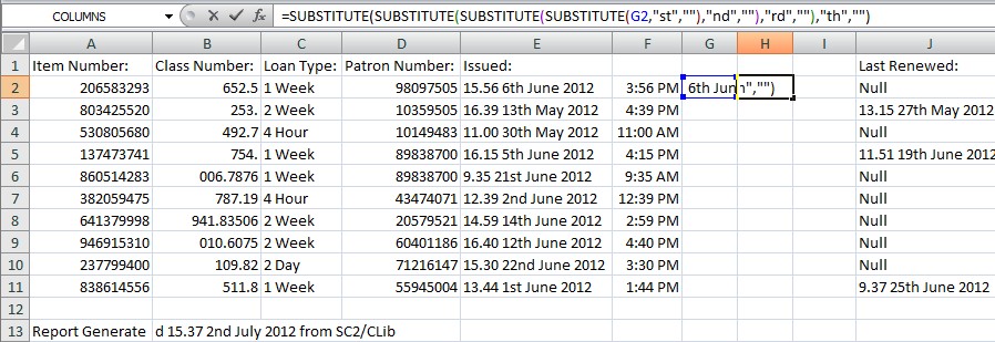
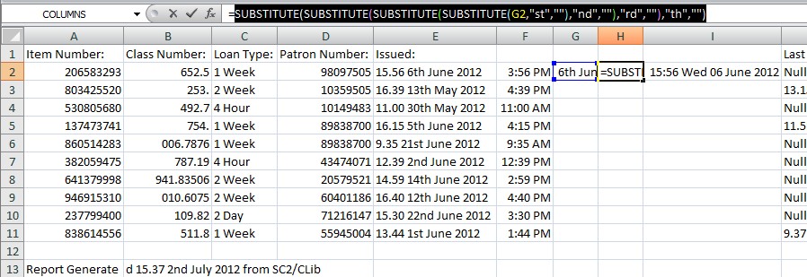
=SUBSTITUTE(SUBSTITUTE(SUBSTITUTE(SUBSTITUTE(G2,"st",""),"nd",""),"rd",""),"th","")
Click H2,
click in the Formula Bar
and modify the formula accordingly, then press Return.
Note that although the "st"
substitution will
abbreviate any Augusts
in our list, Excel can still understand "Augu",
so this is not a problem for us.
29: Format an
Excel-readable Date
In I2 type =DATEVALUE(H2)
(and press Return, as ever). It should now say 12:00 AM in I2 (you may have to expand the
column to see it). This
is because we’ve still got the Time
format from the previous contents
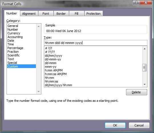
we had in this cell. So right click the cell and select "Format
Cells...", then choose "Custom"
from the "Category:"
list. Delete h:mm
AM/PM from the "Type:"
field and type
hh:mm ddd dd mmmm yyyy
then
click "OK".
Our cell
should now read 00:00 Wed 06
June 2012.
30: Reunite the Date
and Time
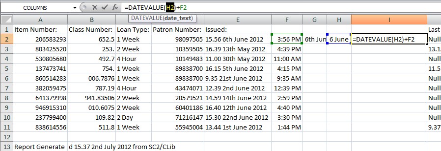
Let's make use of that clock. Click in I2 again and revise the formula
to
=DATEVALUE(H2)+F2 . Now
we have the date and time reunited.
31: Consolidate the
Date Formulae
As we did at step 24, we can nest all the
formulae we’ve used into
the one cell by replacing the cell references in I2 with the formulae in those
cells. So click H2,
highlight and copy all bar the "="
sign from the
formula in the Formula Bar
near the top of the spreadsheet.
You can copy by right-clicking and selecting "Copy" or by using the Ctrl-C
keyboard shortcut. Press Return
to leave the cell, then click I2
and highlight the bit of the formula in the Formula Bar that
says H2.
Paste the contents of the clipboard (right-click and select "Paste" or use the keyboard
shortcut Ctrl-V), and press Return again.
Repeat that for the references to F2
and G2 and we should end
up with:
=DATEVALUE(SUBSTITUTE(SUBSTITUTE(SUBSTITUTE(SUBSTITUTE(MID(E2,6,LEN(E2)),"st",""),"nd",""),"rd",""),"th",""))
+TIME(QUOTIENT(LEFT(E2,5),1),MOD(LEFT(E2,5),1)*100,0)
Assuming we've bolted that formula together properly, we no longer need
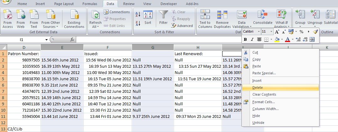
columns F, G and H, so let’s delete them: click
on the F of the column header, drag right to take in G and H, then
right click and select "Delete".
32: Extrapolate the
Date Formula for All Records
Click on cell F2, click
the bottom
right-hand corner and drag down to auto-fill across all our data like
we did in step 26.
33:
Extrapolate the
Date Formula for Renewals
That’s the Issues done. Now let’s do the renewals and returns.
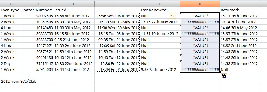
Right-click on the header for column H and select "Insert". Now
highlight F2:F11 and copy.
Click in H2 and paste.
Adjust the
column width to see what we’ve got. It seems that the "Null"s in G2 are
causing us some problems.
34: Anticipate and
Correct Errors using =IFERROR
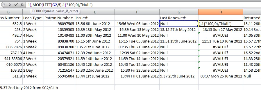
We can solve this "Null" problem by adding a new parameter
to our formula. Click on H2
and then click in the Function
Bar. After
the "=", enter IFERROR( , then
scroll to the end of the formula and type
,"Null") .
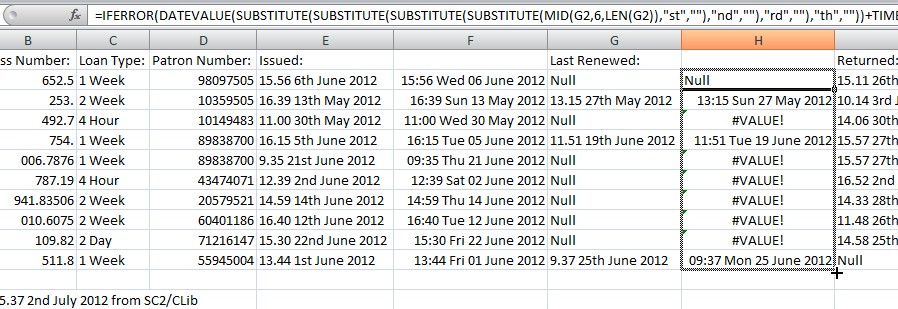
Press Return. H2 should
now
read Null. Click H2 and expand
it to auto-fill our range again.
35: Extrapolate the Date
Formula for Returns
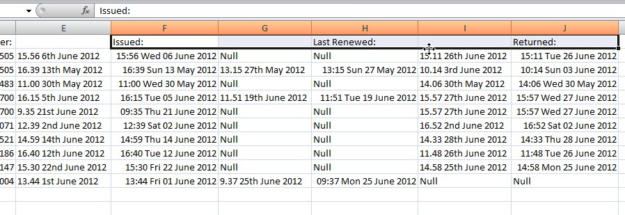
With the range H2:H11
still highlighted, copy the selection. Then
click in J2 and paste.
Adjust the column width to see what we’ve got.
36: Remove Duplication
of Data
We may as well get rid of the duplication we’ve now acquired in our
spreadsheet. Press Escape to remove the copy highlighting in column H.
Click in E2 and drag
across to J11 to highlight
all the dates. Copy and
then Paste Special,
selecting "Values" as
we did in step 10. Next,
select E1:I1. Click along
the middle of the black border of the
selection and drag everything a cell to the right.
Select column E by clicking on the column header. Hold Ctrl and
select columns G and I so that E, G and I are highlighted. Right-click
on the header and select "Delete".
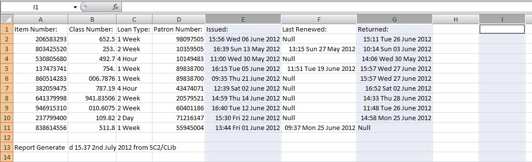
Our spreadsheet should now be
looking not unlike it did after stage 17, but now the dates are Excel
formatted.