VI: Calculate the Fines
In which we use the overdue
calculations to tot up how much we're owed.
46: Thicken the Plot
I shall now throw at you an arbitrary set of rules for our library
which we can employ in our spreadsheet:
a) 4 Hour loans must be returned within 4 hours. Fines are charged at
£1 within the half hour thereafter.
b) 2 Day loans must be returned before the end of the day falling two
days after the book was checked out (three days if checked out on a
Friday; four days if checked out on a Thursday). Fines are charged at
50p per day thereafter.
c) 1 Week loans must be returned or renewed before the end of the day
falling seven days after the book was checked out or last renewed
(eight days if checked out or renewed on a Sunday; nine days if checked
out or renewed on a Saturday). Fines are charged at 20p per day
thereafter.
d) 2 Week loans must be returned or renewed before the end of the day
falling fourteen days after the book was checked out or last renewed
(fifteen days if checked out or renewed on a Sunday; sixteen days if
checked out or renewed on a Saturday). Fines are charged at 20p per day
thereafter.
That should throw a spanner in the works! At first glance it introduces
a pretty hefty headache, but all things can be overcome in Excel.
47: Calculate
Overdues for 4 Hour Loans
Of the above categories, 4 Hour loans are the simplest to deal with.
There are no complications regarding the day the item was checked out.
It's simply a case of whether the thing was returned within four hours.
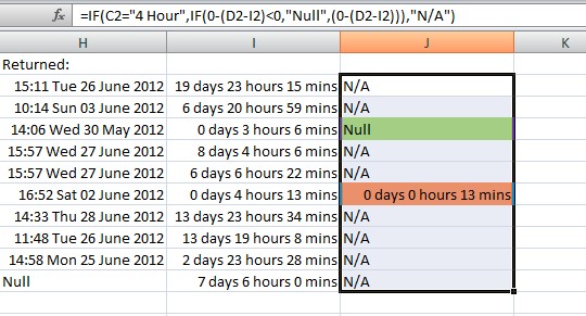
So let’s convert column J to only give the overdue time for 4 Hour
loans. Click in J2 and
amend
the formula to say =IF(C2="4
Hour",IF(0-(D2-I2)<0,"Null",(0-(D2-I2))),"N/A") .
In English: If C2 says "4 Hour" and
0-(D2-I2) is less than 0 (i.e. returned within time), show "Null". If
C2 says "4 Hour" and 0-(D2-I2) is not less than 0 (i.e. overdue), show
the amount of time the item is overdue (0-(D2-I2)). If C2 doesn't say
"4 Hour" show "N/A".
Press Return and then expand this
formula across all our records.
48: Apply
Conditional Formatting to 4 Hour Loan Reports
The introduction of N/A
has messed up
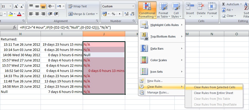
our conditional formatting, so we should sort that out: Highlight J2:J11,
go to "Conditional Formatting"
again and select "Clear Rules
from
Selected Cells" under "Clear
Rules".
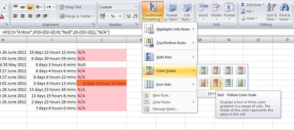
Go back to "Conditional
Formatting", and under "Color
Scales" and select the sixth option
(Red - Yellow Color Scale).
Go back to "Conditional
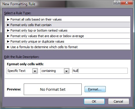
Formatting" once again, and select "New Rule". Click "Format only cells
that contain", choose "Specific
Text" in the first drop-down and type
Null in the field.
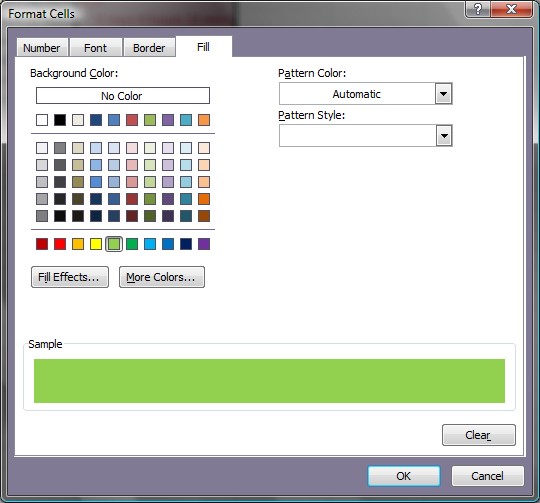
Click "Format", choose
the "Fill" tab, and
pick a
green colour from the palette.
Click "OK" and "OK" again. We should now
have two coloured cells, one orange (with a fine) and one green
(returned on time).
49: Determine the
Base Date for Further Overdue Calculations
The other loan types are more problematic. Let’s attack them in a
new way, piece by piece. We'll start by creating a column that tells us
either the
time the item was checked out or the time it was last renewed.
Type
=IF(G2="Null",F2,G2) into K2 and expand down the column as
usual. Right click and "Format
Cells..." as hh:mm ddd dd mmmm yyyy .
50:
Calculate the
Overdue Threshold for 2 Day Loans
Now
we can think about working out the last possible moment when the item
can be returned without being fined. Let’s start with the 2 Day loan.
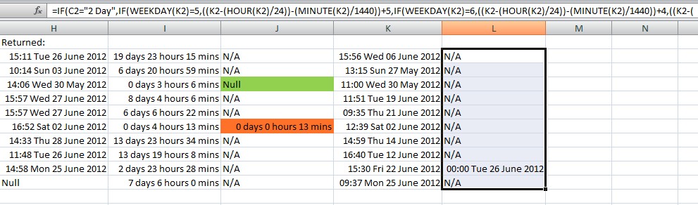
This is the formula we’ll put in L2
(and expand across the rest of
our data):
=IF(C2="2
Day",IF(WEEKDAY(K2)=5,((K2-(HOUR(K2)/24))-(MINUTE(K2)/1440))+5,
IF(WEEKDAY(K2)=6,((K2-(HOUR(K2)/24))-(MINUTE(K2)/1440))+4,((K2-(HOUR(K2)/24))-(MINUTE(K2)/1440))+3)),"N/A")
WEEKDAY identifies a day of the week in our datevalues. WEEKDAY(K2)=1
is true if K2 is a Sunday, WEEKDAY(K2)=2 is true if K2 is a Monday,
etc.
A user has all day to return the book, so we need to set our clocks to
midnight. (K2-(HOUR(K2)/24))-(MINUTE(K2)/1440) does just that. HOUR
gets the hour from the datevalue in K2, but datevalues work in days, so
we divide the hour value by 24 before taking it away from the
datevalue. Likewise, we divide the minute value by 1440 (24 hours x 60
minutes). Once the clock is zeroed we can add the number of days the
item is allowed out: 5 for a Thursday, 4 for a Friday, and 3 for
anything else.
In English, then, the formula says: If
C2 says "2 Day" and the day in K2 is Thursday, we get the date in K2
minus the hours and the minutes given in K2 but plus 5 days. If C2 says
"2 Day" and the day in K2 is Friday, we get the date in K2 minus the hours and
the minutes given in K2 but plus 4 days. If C2 says "2 Day" and the day
in K2 is any day exept Thursday or Friday, we get the date in K2 minus the hours and
the minutes given in K2 but plus 3 days. If C2 doesn't say "2 Day" we
get "N/A".
Format the cells as hh:mm ddd dd mmmm yyyy .
51:
Calculate
Overdues for 2 Day Loans
Having got the exact moment when the
item must be returned, we can
look to see if any of our items in this loan category have come back
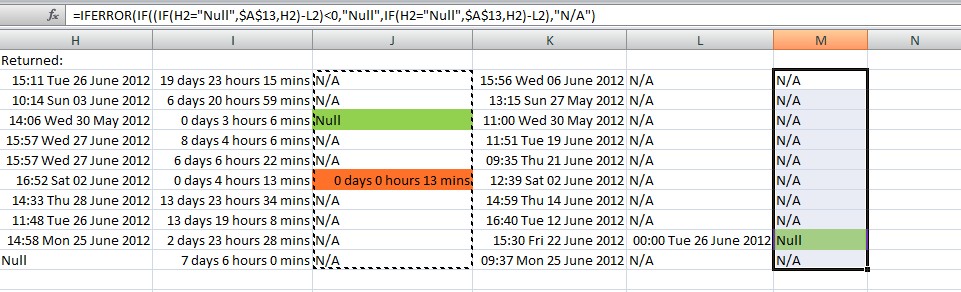
late. In M2 we can type:
=IFERROR(IF((IF(H2="Null",$A$13,H2)-L2)<0,"Null",IF(H2="Null",$A$13,H2)-L2),"N/A")
If
H2 says "Null", if A13-L2 is less than 0, say "Null", otherwise say
A13-L2. If H2 doesn't say "Null", if H2-L2 is less than 0, say "Null",
otherwise say H2-L2. If we get an error, say "N/A".
Expand this down to M11.
52:
Apply
Conditional
Formatting to 2 Day Loan Reports
We should probably give this the same
formatting as J2:11.
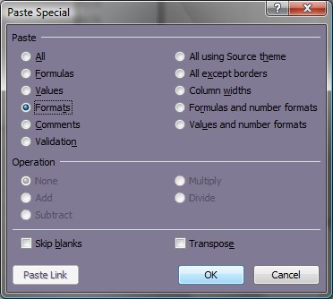
Highlight J2:11 and copy
the cells. Now highlight
M2:11 and select "Paste Special". Choose "Formats" on the radio
buttons
and click "OK".
M10 should now be green.
53: Calculate Overdues
for 1 Week Loan Items
We can rework steps 50-52 for the other two loan
types. Have a go
yourself first. It may be helpful to copy the formulae from the 2 Day
loans and modify them accordingly. Calculate the last due date for a 1
Week
loan in N (cf. step 50), and the corresponding
overdues in O (cf. step
51).
What you come up with should look like this:
N2:
=IF(C2="1
Week",IF(WEEKDAY(K2)=7,((K2-(HOUR(K2)/24))-(MINUTE(K2)/1440))+10,
IF(WEEKDAY(K2)=1,((K2-(HOUR(K2)/24))-(MINUTE(K2)/1440))+9,((K2-(HOUR(K2)/24))-(MINUTE(K2)/1440))+8)),"N/A")
O2:
=IFERROR(IF((IF(H2="Null",$A$13,H2)-N2)<0,"Null",IF(H2="Null",$A$13,H2)-N2),"N/A")
54: Calculate
Overdues for 2 Week Loan Items
Now do the same for the 2 Week loans in P and Q.
P2:
=IF(C2="2
Week",IF(WEEKDAY(K2)=7,((K2-(HOUR(K2)/24))-(MINUTE(K2)/1440))+17,
IF(WEEKDAY(K2)=1,((K2-(HOUR(K2)/24))-(MINUTE(K2)/1440))+16,((K2-(HOUR(K2)/24))-(MINUTE(K2)/1440))+15)),"N/A")
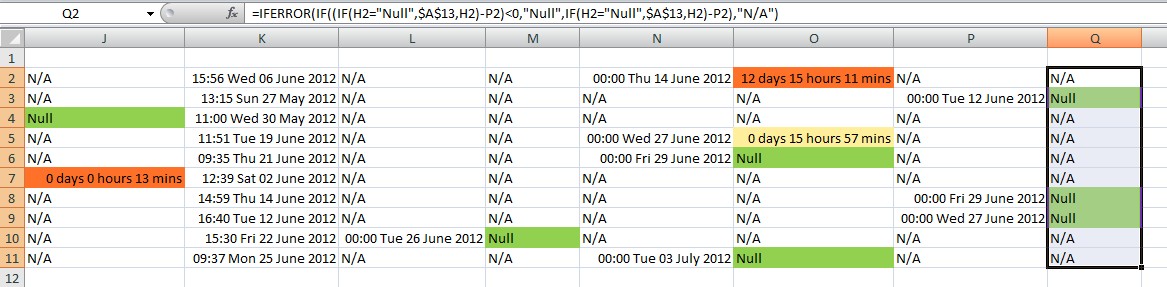
Q2:
=IFERROR(IF((IF(H2="Null",$A$13,H2)-P2)<0,"Null",IF(H2="Null",$A$13,H2)-P2),"N/A")
55: Apply Conditional
Formatting to 1 & 2 Week Loan Reports
Format the data as we did in step 52. Our
spreadsheet should now look
something like this:
56: Create a Combined
Overdue Report
We can make a combined column of overdue statuses in R if we like.
Have a go at working out a method using the IF function.
You should end up with something like
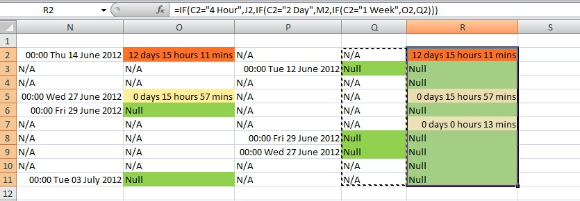
(but not necessarily the same as) this in R2:
=IF(C2="4
Hour",J2,IF(C2="2 Day",M2,IF(C2="1 Week",O2,Q2)))
Format the data as before and it should look like this:
57: Calculate Fines for
Overdue Items
Now, at last, we can calculate our fines. Here’s what we need to
put in S2 and expand
across the rest of the rows:
=IFERROR(IF(C2="4
Hour",ROUNDUP(J2*48,0),IF(C2="2 Day",(ROUNDUP(M2,0))/2,
IF(C2="1
Week",(ROUNDUP(O2,0))/5,(ROUNDUP(Q2,0)/5)))),"Null")
ROUNDUP does what it says (the 0 in the formula is the number of
decimal places to which we're rounding). In the case of the 4 Hour loan
we’re
fining within the half-hour, so we multiply our datevalue by 48 (the
number of half-hours in a day). In the rest of the cases we’re fining
by the day so we don’t need to change the datevalue, but we do need to
divide our rounded figure to get the 50p ((ROUNDUP(M2,0))/2) and 20p
((ROUNDUP(M2,0))/5) rates.
If
C2 says "4 Hour", round up J2*48. If C2 says "2 Day", round up M2 and
divide by 2. If C2 says "1 Week" round up O2 and divide by 5. If C2
says anything else, Round up Q2 and divide by 5. If we get an error,
give "Null".
58: Collapse Grouped Data
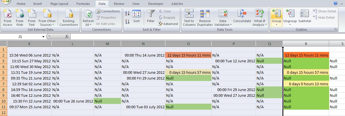
We don’t really need to look at columns I to Q so select them all
(click on the header of column I and drag to column Q), go to the
"Data" ribbon and click
on "Group" in the "Outline" menu.
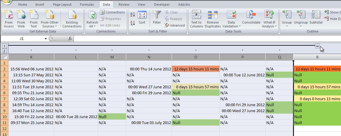
This brings
up a new bar at the top of our sheet and we can click on the minus sign
to collapse the columns out of sight.
59: Tidy Things Up a Bit
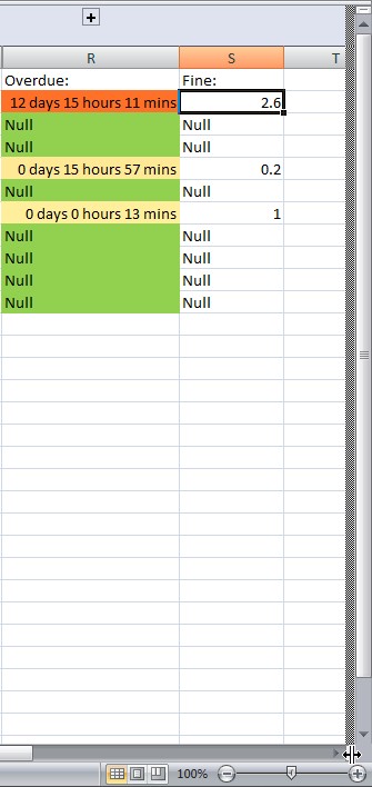
In R1 type Overdue: and
in S1 type Fine: . Now click
on the little
rectangular toggle in the bottom right of the screen, at the right-hand
end of the horizontal scrollbar.
Drag it into the spreadsheet and you
will see that it is going to create a divider. Place the division
between columns E and F. Arrange the panels so that "Item Number:" is
our left-most column, and "Fine:"
is our right-most. This will allow us to see what we're doing if we're
at a low resolution.
60: Format the Fines and
Use Them Wisely
Copy the formatting from R2:R11
and paste it into S2:S11.
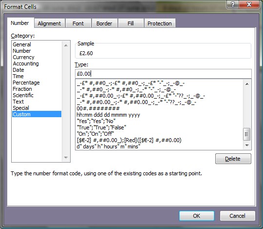
We now
need to convert the data in this column to a currency format. Right
click and select "Format
Cells...". Choose "Custom"
and then type
£0.00 in the "Type:"
box before clicking "OK".
Look in the bottom
corner of the spreadsheet, where it says "Sum:". We’ve made £3.80.
Quick, let’s go and spend it on gin! We’ve earnt it!