V: Calculate the Overdues
In which we start to do some sums at
last in order to determine which items were overdue.
37: Add
Another Column
Now let’s look at column C. We have four different loan categories
so let’s make them into something compatible with our newly formatted
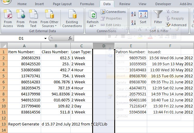
dates. First things first, let’s add a new column between C and D. We
should’ve got the idea of how to do this now (we last did it at step
33).
38: Extract Loan
Period Data using =IF
We can convert the loan categories to time periods using a
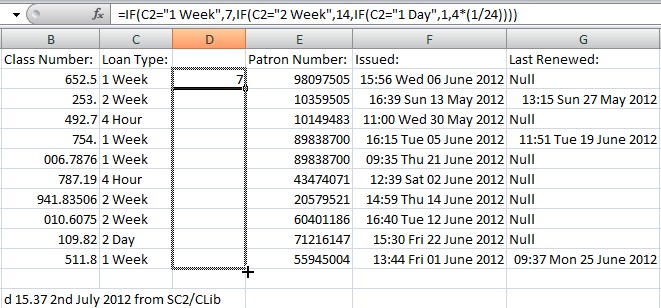
conditional formula type. Let’s go with IF. Click D2 and type:
=IF(C2="1
Week",7,IF(C2="2 Week",14,IF(C2="1
Day",1,4*(1/24))))
This
should
cover all eventualities: If C2=1 Week we get 7 days in D2. Likewise, 2 Weeks gives 14 and 1 Day gives 1. Any other value in C2 returns 4*(1/24), that is 4
hours.
Having typed in the formula, press Return and we should get a 7 in D2.
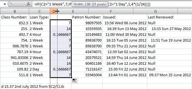
Now expand the cell to auto-fill down to D11.
39: Merge Header
Cells
Adjust the column width for D to about 25 pixels: just wide enough
to see the numbers.
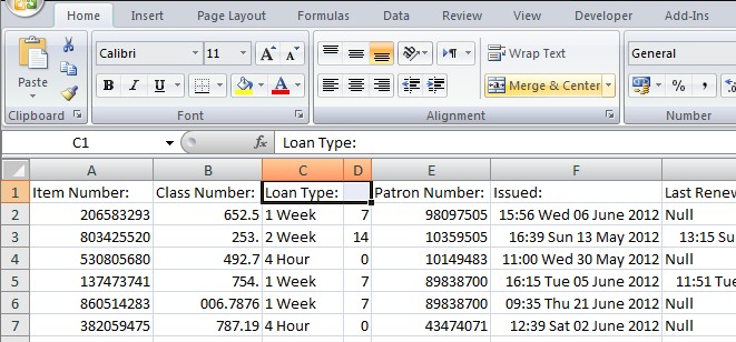
Select C1 and D1 and the click "Merge &
Center"
from the "Alignment" menu on the "Home" ribbon. This combines the two
cells into a unified header for both columns.
Adjust the width of
column C to neaten things up and make some more room.
40: Calculate Loan
Duration using =IF
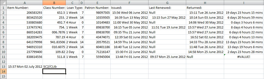
Now let’s think about doing some maths. In I2 type
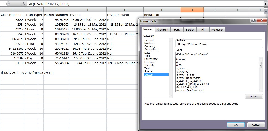
=IF(G2="Null",H2-F2,H2-G2) and press Return. If the item’s
not been
renewed, the content of I2
will be the number of days between the item
being checked out and being returned (H2-F2). If renewed, it’s the
number of days between the renewal and the return (for this exercise we
shall assume that
the system does not allow renewals on late items).
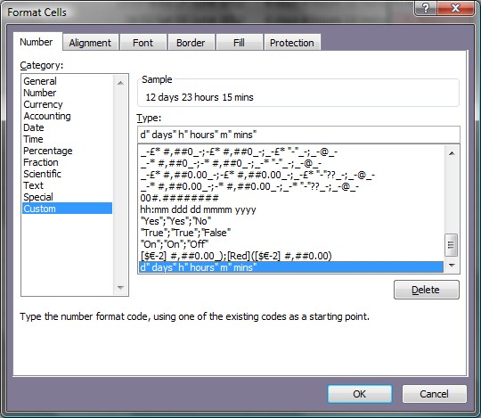
Right click on I2 and
select "Format Cells...".
Choose "Custom" and
enter d" days"
h"
hours" m" mins" , then click "OK".
Now drag to
auto-fill our cells across all of our rows.
41: Create a
Reference Cell for the Report Date
We’ve got a #VALUE!
error in cell I11 because
this item is still
out, so we need to ammend our formula so that the loan duration on
unreturned items is calculated by some other means. We could use
today’s date and time as a reference by using the formula =NOW() , but
given we’ve got a date label for when the report was generated we
should probably use that instead. The data we need is in cell B13. We
could extract it using methods like those we employed in steps 19 to
35, but it’s
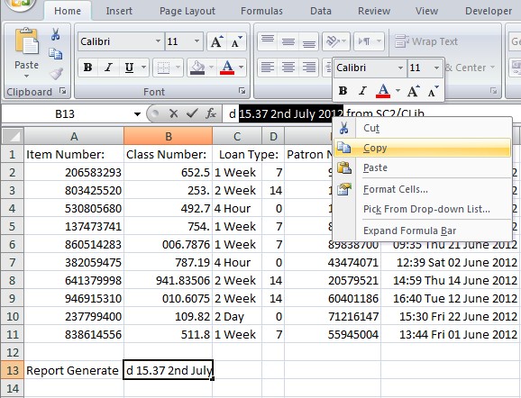
only the one date so it seems an unnecessary palaver. Instead, click in
B13 and
copy 15.37 2nd July 2012
from the Formula Bar.
Press Escape to leave the forumla.
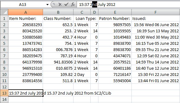
We may as well paste what we've copied into A13 because the text currently
in there is not much use to us. Once
pasted, change the . to a :
in the Formula Bar, and
delete the nd
. Then press Return.
The result is
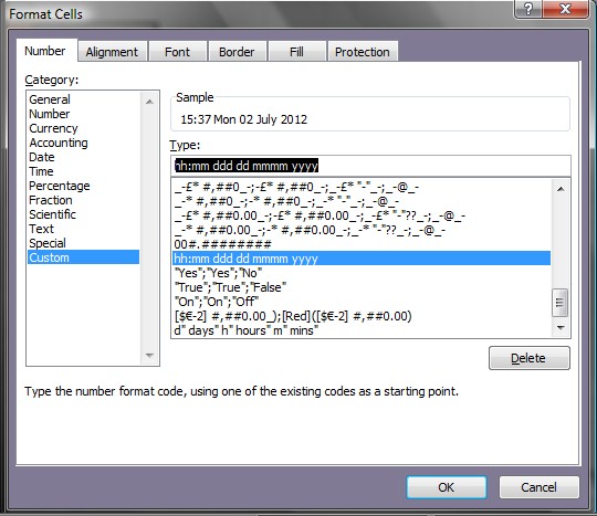
a lovely date that Excel can read. Right click A13 and select "Format Cells...". Sroll down
the the list of formats under the "Type:" box and pick hh:mm ddd dd mmmm
yyyy then click "OK".
While we’re at it, let’s delete
everything from B13 except
SC2/CLib which we’ll keep
for reference. Adjust the column widths if needs be to neaten things up
a little.
42: Repair the Loan
Duration Formula using =IFERROR
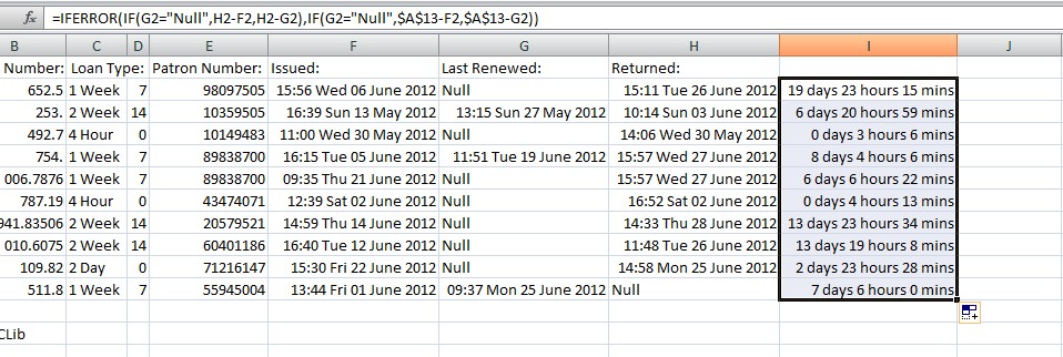
We now have a fixed reference date we can use it in our formula in
column I, so let's use it. Click I2
again and edit the formula to read
=IFERROR(IF(G2="Null",H2-F2,H2-G2),IF(G2="Null",$A$13-F2,$A$13-G2))
In English, this translates as:
If G2 says "Null", take the date in
F2 away from the date in H2, otherwise take the date from G2 away from
the date in H2. If this sum results in an error, try this instead: If
G2 says "Null", take the date in F2 away from the date in A13,
otherwise take the date from G2 away from the date in A13.
We
use the $ signs to
create a fixed cell reference rather than a relative
one, otherwise, when we expand the formula into I3, it would look for
data in A14.
Press return to enter the formula, and then expand it across all of our
rows so that we can
correct the error in I11.
We should give this column a title, too. Type Loan Duration:
in I1.
43: Calculate
Overdues
We should now have everything in place to detect any items which
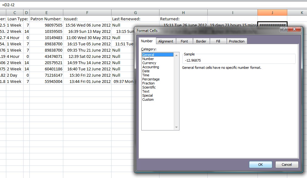
are overdue or which were returned overdue. Click J2 and type =D2-I2
and press Return. We get a load of hash, and no amount of column
movement will reveal anything. This is because we’ve generated a
negative date and Excel can’t handle that. So right-click, select
"Format Cells..." and
choose "General" from
the "Category:" list
before
pressing "OK".
Now fill down to J11.
44: Highlight
Overdues using Conditional Formatting
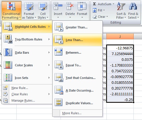
With J2:J11 still
highlighted, go to "Conditional
Formatting" on
the "Styles" menu of
the "Home" ribbon.
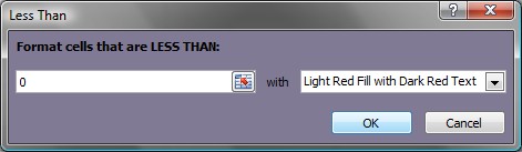
Under "Highlight Cells Rules"
click "Less Than...".
Type 0
in the first field of the dialogue box, and click "OK".
The overdue items are now highlighted red.
45: Format Overdues
as a Duration
Let’s come up with a way of making this column a bit more readable.
Click J2 and amend the
formula to read
=IF(0-(D2-I2)<0,"Null",(0-(D2-I2))) . The "0-"es here will convert any
negatives to positive, and any items returned within time will be
marked as Null. Press
Return, then drag J2 to
expand the formula across all the records. Now go to
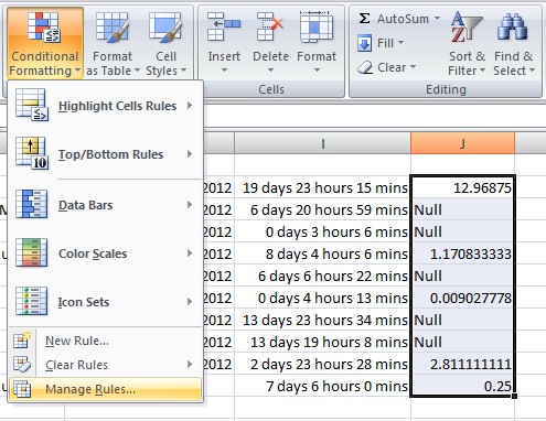
"Conditional Formatting"
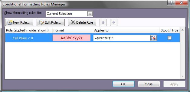
and select "Manage Rules".
Double-click
where it says "Cell Value <
0".
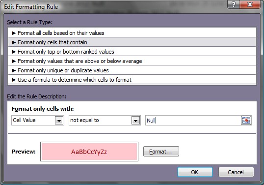
In the "Edit Formatting Rule"
dialogue, change the second drop-down to
say "not equal to" and
type Null
in the blank field.
Click "OK" and
"OK" again.
Right click on the array and select "Format Cells...", go to
"Custom", scroll down
and pick the d"
days" h" hours" m" mins" form we
put in before.
Click "OK" again and we
have a nice, neat overdue report.